By the end of this module, you’ll gain experience in dealing with all the data that your applications will need to generate and consume.
Module videos:
Data (More Specifically - of the Big Variety)
Module video: Big Data Overview [14:10]
It is now time to discuss data, or more commonly, that thing you have to deal with on a daily basis. Data can be anything, from user input to usage patterns to consumed weather data. Your cloud applications will most likely be managing data of some kind.
If you’re in the cloud realm, there is a reasonable chance that your data is going to be “big.” Big data is a very timely topic, however its definition is constantly changing (mainly due to the result at which data changes). Previously, data was in the gigabyte range to be considered “big.” Now, we’re in the peta/zetabyte range and need to be able to deal with absolutely massive streams of information. Figure 1 (c/o Google) shows you a nice little visualization of what we mean by “big.”
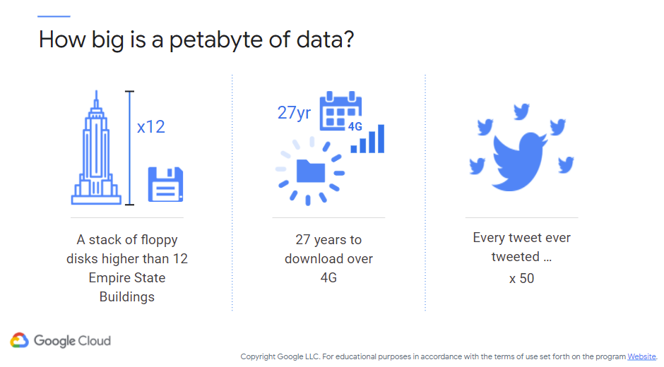
Figure 1: Petabyte Size
That’s talking about petabytes. Already in the various big data-related outlets they’re discussing zetabytes of data (hint: a scale factor more than petabytes). That is how much data you have to deal with. However, a petabyte really isn’t all that much at scale. Figure 2 (c/o Google) shows how little data can be stored within a petabyte:
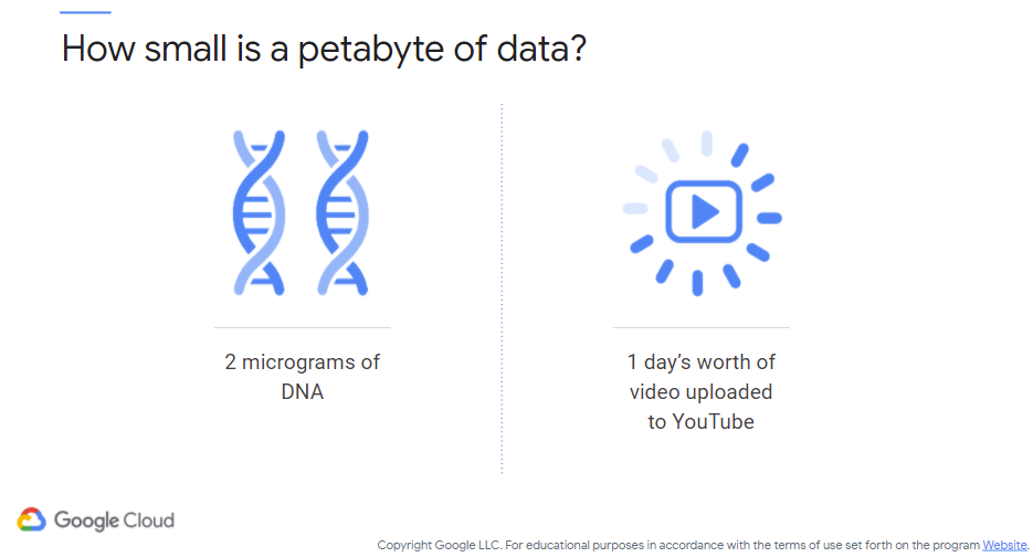
Figure 2: Petabyte Size - Inverted
Before we talk about the cloud services we can use to manage and analyze our data, let’s talk about the other factors that comprise big data. The following image (c/o Edureka) presents a pretty reasonable overview of the more “standard” V’s that big data is known for:
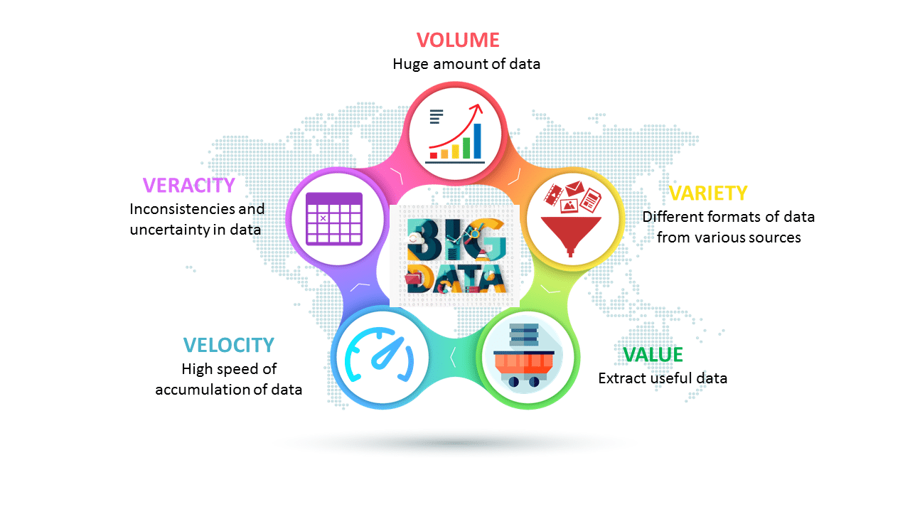
5 V’s of Big Data (c/o Edureka)
Some places list way more V’s, some way less, though 5 is typically accepted as representative of big data. The reason why we call them “V’s” should be clear – they all start with V.
- Volume
Big data, at its heart, means that there is a massive amount of information to store, analyze, and sift through. A standard SQL installation will typically falter with this amount of data. Again, we’re in the peta/zetabyte range (as of 2021 anyway).
- Velocity
Velocity is the speed at which data comes in and leaves our applications. Consider the various social media platforms and all of the live posts, updates, photos, videos, etc. that are constantly being posted by everybody worldwide. The speed at which the underlying applications must handle that data (e.g., how do you quickly and reliably pull up your friend information such that the user doesn’t notice the lag in searching for a SELECT * FROM FRIENDS WHERE ID='you' type of search? If you don’t know what I’m getting at, the prior SQL-ish search would be super-slow for a large amount of data.
- Variety
One consideration for big data is that the format of the data is generally open to interpretation. In normal database applications you enforce a schema that formats each table. Big data is generally schema-less (i.e., NoSQL-type applications) as we don’t necessarily know in which format the data will be arriving (and/or leaving). Data could be an image, a sensor value, a long-winded blog post. It is up to your applications to handle the data and format it appropriately.
- Veracity
Do you trust the data coming in? Is it possible that it is malformed, or worse, malicious? With large amounts of streaming data from multiple sources you will need to ensure that there is little to no uncertainty in your data, as that can very quickly corrupt your database and/or application! Maybe there are inconsistencies resulting from the same data reported from multiple sources. Your application must be prepared for this!
- Value
This is the “business/marketing” side of big data, however also very very important for those companies concerned with the business of data analytics. Without diverting into the deep, dark field of analytics, Value effectively means what you are able to get out of your data. Specifically, what business decisions can we make as a result of analyzing the data? Is our data valuable or worthless (and do we keep it if it is worthless?).
Fortunately, the Cloud
As you would expect by this point, there are several cloud services to help us manage big data for our applications. Per usual, we’ll talk about them in terms of Google Cloud, however similar services exist in Azure/AWS. We’ll be mainly looking at this in terms of managed services (mild shock) that we can leverage to do all the heavy lifting for us. Here are the main services we’ll be looking at in Google Cloud (with their other provider analogues):
- Dataproc
- Amazon analogue = AWS EMR
- Microsoft analogue = Azure Hindsight
Dataproc (and similar) are going to be your engines for processing big data. Common strategies leverage Hadoop/Spark for working with data. These are open-source technologies that can be used for handling massive amounts of unstructured data.
- Dataflow
- Amazon analogue = AWS Glue (formerly Data Pipeline)
- Microsoft analogue = Azure Data Factory
You may be interested in streaming data. Streaming data effectively has you analyze and manage data as it arrives in real time, and can typically be setup as a streaming or batch processing service.
- BigQuery
- Amazon analogue = AWS Redshift
- Microsoft analogue = Azure Synapse Analytics
You will also probably need to manage analytics at some point as well (or, analyzing your data). Essentially, you will take what you know of common database queries (think: SQL) and translate them to higher-order services for quickly searching for, understanding, and leveraging your data. Data warehousing was the precursor to this area.
Dataproc
First of all, let’s talk about Hadoop and Spark (both open-source projects from Apache). You will often find these two technologies in big data applications. Hadoop effectively ties together computers/servers in a cluster to enable distribution and processing of data, and Spark is an analytics engine for large-scale data processing (both in stream form and batch form). Dataproc then ties these two technologies together as a managed service. With Dataproc clusters can be spun up quickly, managed, and run in an ephemeral fashion (i.e., you save money when they’re off). Figure 3 (c/o Google) shows an overview of Dataproc and its sub-services:
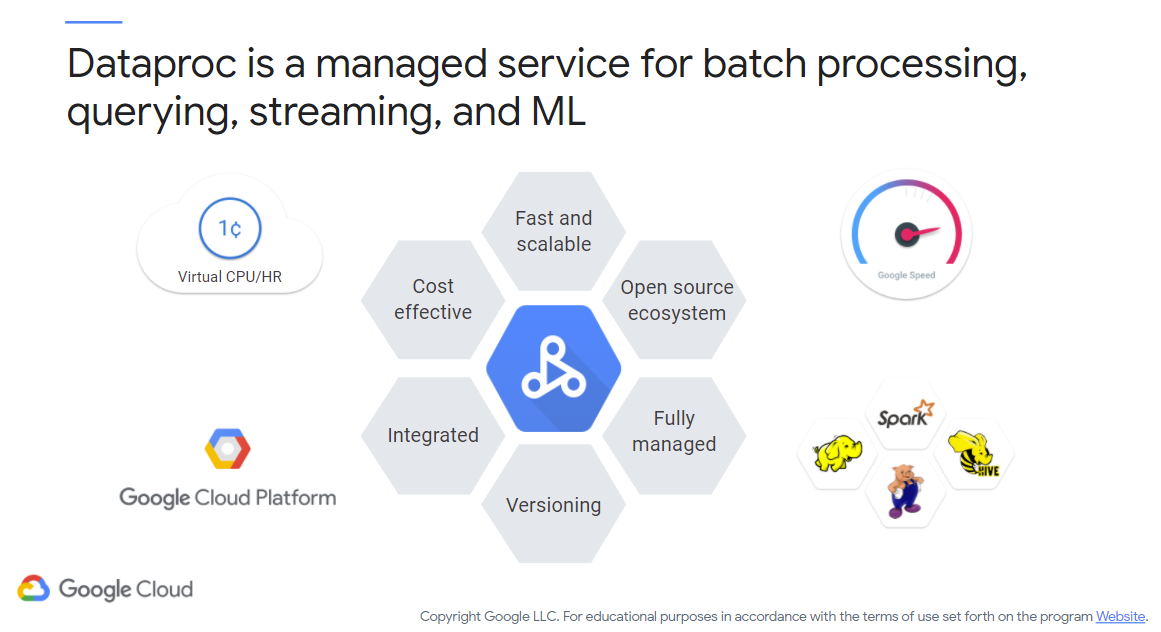
Figure 3: Dataproc Overview
Here are some quotes from Google on the key Dataproc features:
Dataproc is priced at 1 cent per virtual CPU per cluster per hour, on top of any other Google Cloud resources you use. In addition, Dataproc clusters can include preemptible instances that have lower compute prices. You use and pay for things only when you need them.
Dataproc clusters are quick to start, scale, and shutdown, with each of these operations taking 90 seconds or less, on average. Clusters can be created and scaled quickly with a variety of virtual machine types, disk sizes, number of nodes, and networking options.
You can use Spark and Hadoop tools, libraries, and documentation with Dataproc. Dataproc provides frequent updates to native versions of Spark, Hadoop, Pig, and Hive, so there’s no need to learn new tools or APIs, and it’s possible to move existing projects or ETL pipelines without redevelopment.
You can easily interact with clusters and Spark or Hadoop jobs, without the assistance of an administrator or special software, through the Cloud Console, the Cloud SDK, or the Dataproc REST API. When you’re done with a cluster, simply turn it off, so money isn’t spent on an idle cluster.
Image versioning allows you to switch between different versions of Apache Spark, Apache Hadoop, and other tools.
The built-in integration with Cloud Storage, BigQuery, and Cloud Bigtable ensures data will not be lost. This, together with Cloud Logging and Cloud Monitoring, provides a complete data platform and not just a Spark or Hadoop cluster. For example, you can use Dataproc to effortlessly ETL terabytes of raw log data directly into BigQuery for business reporting.
Figure 4 (c/o Google) shows the “typical” Spark/Hadoop workflow you might use if you weren’t looking to the cloud for service management.
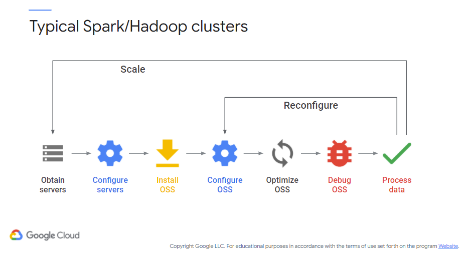
Figure 4: Typical Spark/Hadoop Workflow
Essentially, you are in charge of managing and configuring your infrastructure and services, optimizing and debugging for your particular needs, and only then running your big data processing applications. Dataproc mimics the above flow, however the process is managed by Google (or your provider) to support your needs. This process not only reduces the infrastructure overhead but also the cost. If you recall, all these services are ephemeral, meaning that they’ll be running efficiently and cost-effectively (or, as needed).
Another nice aspect is that the compute and storage aspects are neatly separated, whereas in traditional deployments it is possible that they are on the same server. If a server is down for maintenance for some reason, then there is the chance that your data is unavailable as well. In Dataproc storage is handled via Cloud Storage, enabling that neat separation. Another benefit is that the time from job submission to start is very small (approximately 90 seconds on average) resulting from this separation as well.
Dataproc Workflows
Figure 5 (c/o Google) shows the relationship between cluster, job, and output. Here, you can see how the cluster agent fit together to create jobs (of varying types), resulting in the outputs you need for your cloud applications.
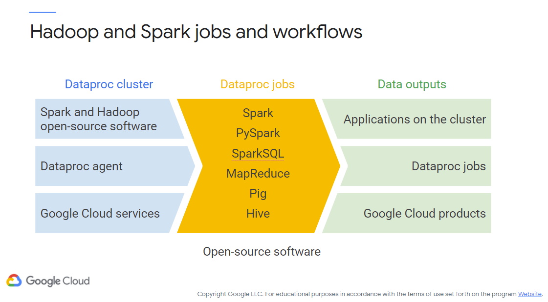
Figure 5: Spark/Hadoop Jobs
Next, Figure 6 (c/o Google) shows the specific cloud services that are used for each aspect of Dataproc, from your data source to monitoring to analytics. Depending on the compute/query you need to perform, there is a managed service that can be used to support your application. For instance, if you need to log or monitor your job Cloud Logging/Cloud Monitoring could be used, respectively (in addition to whatever else you prefer).
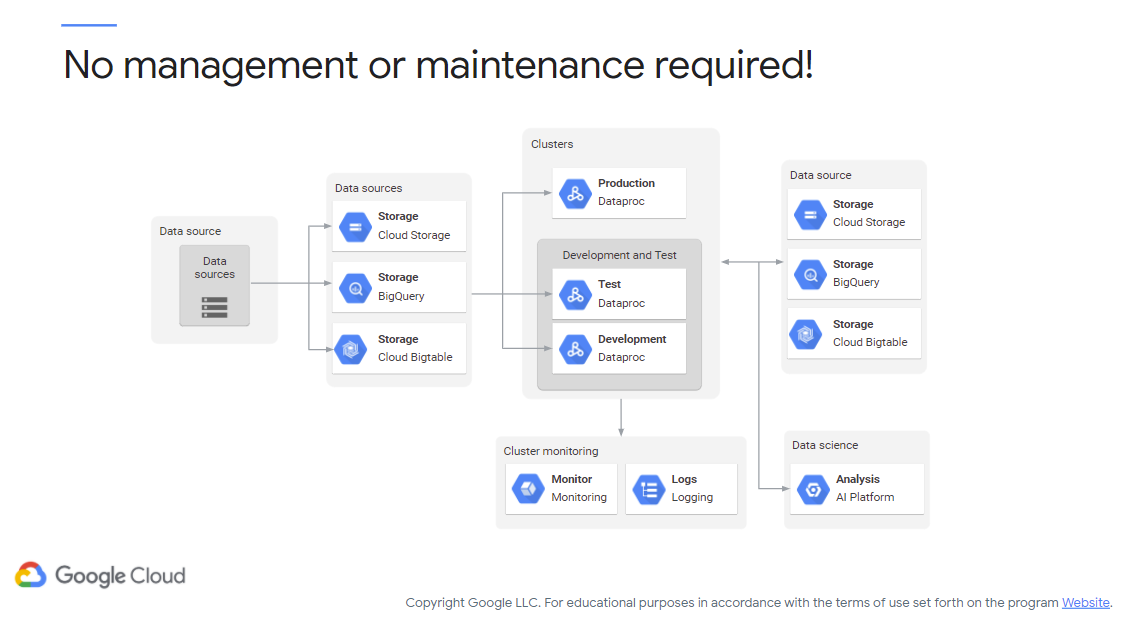
Figure 6: Dataproc Pieces
Next, you’ll be blasted with a series of slides and quotes from Google, as they provide guidance on how to use Dataproc in various situations you will indubitably find yourself in.
Dataproc Use Cases
Quote warning: this all comes directly from Google (yet the advice is still applicable for AWS/Microsoft).
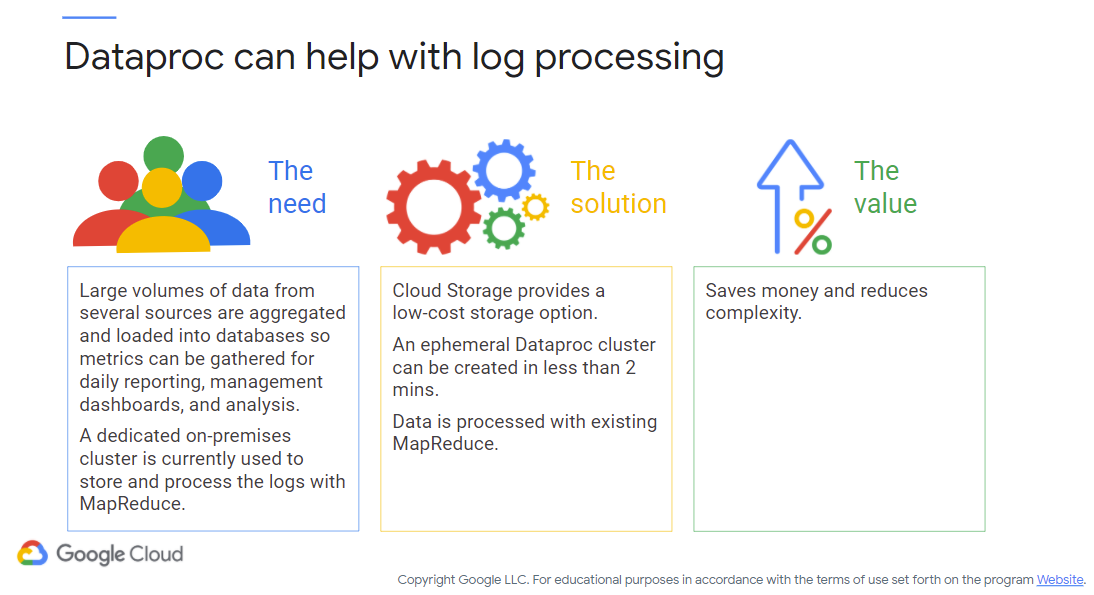
Figure 7: “Dataproc/Log Processing”
Let’s look at a few use cases. In this example, a customer processes 50 gigabytes of text log data per day from several sources, to produce aggregated data that are then loaded into databases from which metrics are gathered for daily reporting, management dashboards, and analysis. Up until now, they have used a dedicated on-premises cluster to store and process the logs with MapReduce.
So what’s the solution? Firstly, Cloud Storage can act as a landing zone for the log data at a low cost. A Dataproc cluster can then be created in less than 2 minutes to process this data with their existing MapReduce. Once completed, the Dataproc cluster can be removed immediately.
In terms of value, instead of running all the time and incurring costs even when not used, Dataproc only runs to process the logs, which saves money and reduces complexity.
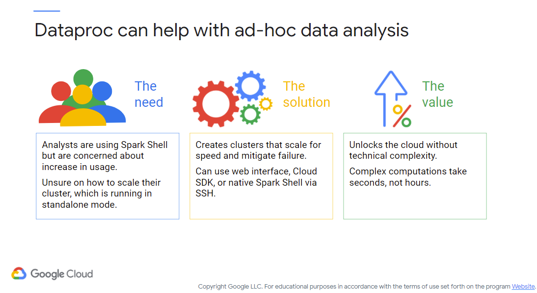
Figure 7: “Dataproc/Ad Hoc Analysis”
In this organization, analysts rely on, and are comfortable using, Spark Shell. However, their IT department is concerned about the increase in usage, and how to scale their cluster, which is running in Standalone mode.
As a solution, Dataproc can create clusters that scale for speed and mitigate any single point of failure. Since Dataproc supports Spark, Spark SQL, and PySpark, they could use the web interface, Cloud SDK, or the native Spark Shell via SSH.
In terms of value, Dataproc quickly unlocks the power of the cloud for anyone without added technical complexity. Running complex computations now take seconds instead of minutes or hours.
- Additional information on Spark Shell
- Additional information on Spark Standalone Mode
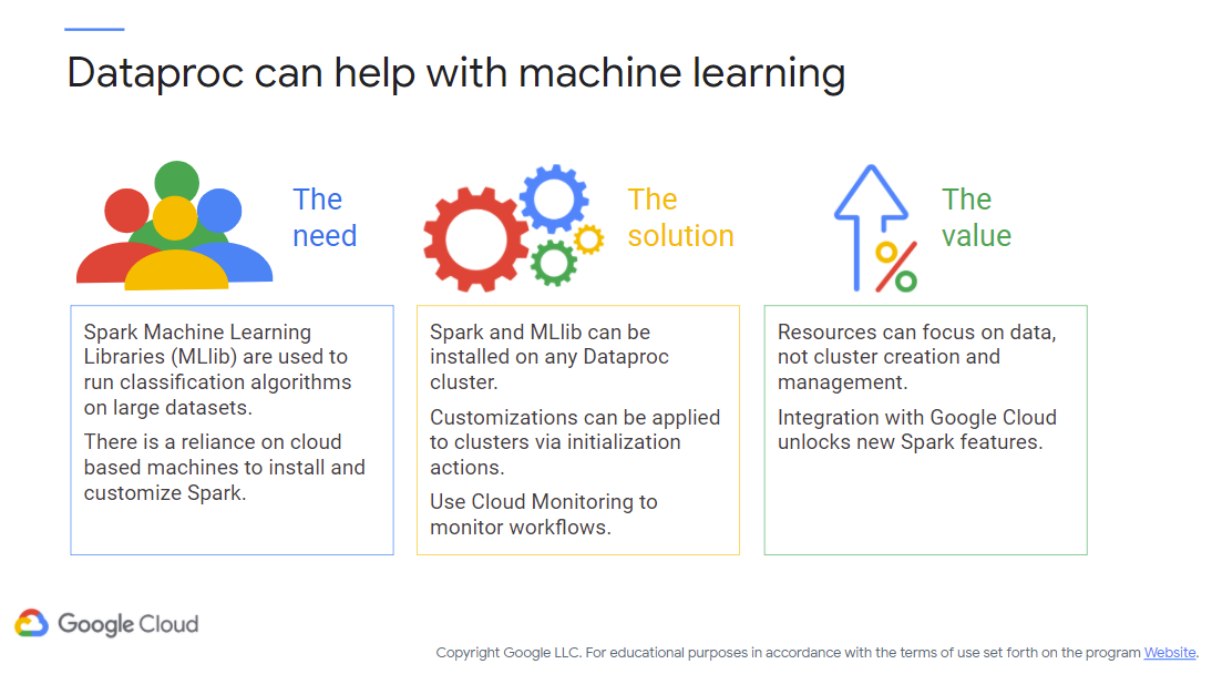
Figure 8: “Dataproc/Machine Learning”
In this third example, a customer uses the Spark Machine Learning Libraries (MLlib) to run classification algorithms on very large datasets. They rely on cloud-based machines where they install and customize Spark.
Because Spark and the MLlib can be installed on any Dataproc cluster, the customer can save time by quickly creating Dataproc clusters. Any additional customizations can be applied easily to the entire cluster through initialization actions. To keep an eye on workflows, they can use the built-in Cloud Logging and Monitoring.
In terms of value, resources can be focused on the data with Dataproc, not spent on cluster creation and management. Integrations with new Google Cloud products also unlock new features for Spark clusters.
- Additional information on the Spark Machine Learning Libraries (MLlib)
Here is a workthrough of a Codelab involving Dataproc and Spark – setting up a Jupyter notebook environment!
Ok, enough preamble. Let’s do some Dataproc work!
Lab choices
For this assignment you have a choice! You can either do the Qwik Start with templates or Python (or both, but I’ll only be grading you on one!). See Blackboard for submission details.
And you have to do this one regardless!
Dataflow (or, how I learned to stop worrying and love the datastream)
NO MOM, IT’S NOT A DATED REFERENCE THEY’LL UNDERSTAND. ಠ_ಠ
Time to talk about a massive pipeline of data flowing through your applications! Dataflow is based on Apache Beam and support workflows such as extract-transform-load, batch, and streaming. Dataflow can be used to build pipelines for data, including monitoring and analysis. Nicely, these pipelines support batch and stream processing, so you are able to specify your preferred method of data ingress/egress. As with all Google Cloud services, scalability and on-demand access are built in to support your needs.
If you want to extend your data pipeline, you can incorporate it with other cloud services, including logging, Cloud Storage, Pub/Sub, BigQuery, and even external services such as Apache Kafka and HDFS.
There are also pre-baked templates for you to select to get quickly up and running with Dataflow, including streaming and batch templates. Figure 9 (c/o Google) shows some of those that are available.
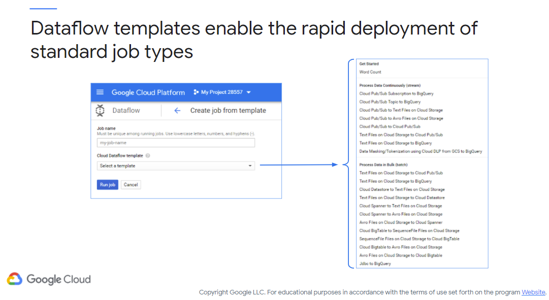
Figure 9: Dataflow Templates
One of the side benefits of using templates is the reduction in effort for pipeline code development and management. But what is a pipeline you ask? Well..
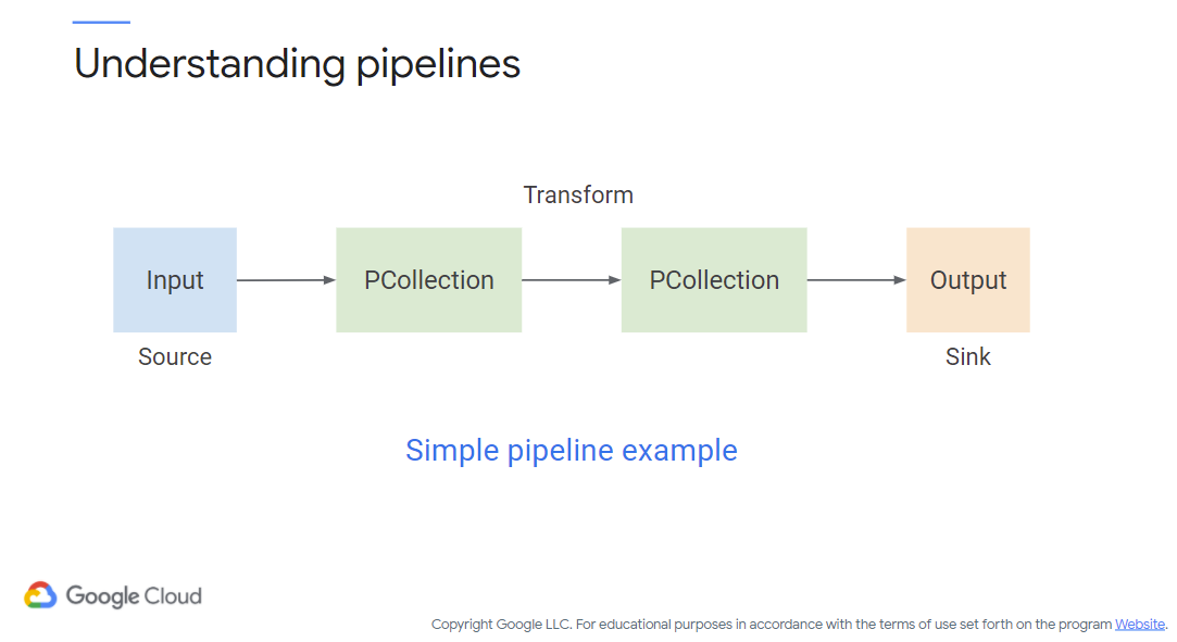
Figure 10: A pipeline (c/o Google)
A pipeline is a complete process on 1+ datasets, starting from a source (of some data) and ending with a sink (where your data is going to). Along the way there may be a series of transformations applied to finesse/understand the data (e.g., filter, join, aggregate, etc.). The data may also be shaped into a form understandable by your application(s). The sink is where the data needs to end up – either internal to Google Cloud, external to some other location, or even your original source! The pipeline is typically modeled as a directed acyclic graph (DAG).
In the figure you also see a PCollection. This object is a container of near-unlimited size representing the data within the pipeline. They can be bounded or unbounded and represent the inputs/outputs to transformations. A transformation acts on one or more PCollections, transforming each piece of data in that collection, and then deliver a new PCollection as output.
Sources/Sinks generally have an API that provide the capabilities for reading data into and out of a pipeline. For Google Cloud Dataflow, you have the ability to use built-in sinks/sources or provide your own custom interface.
Figure 11 (c/o Google) shows a pipeline with multiple transform paths with a bit more detail on what can be inside of a PCollection:
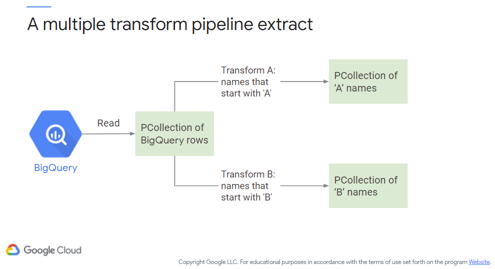
Figure 11: Dataflow - Multiple Paths
Note here that the transform is essentially filtering based on the first letter of a name. We assume a sink exists along this pipeline, however it is not shown here for presentation purposes. Figure 12 (c/o Google) next shows an additional transform (flatten) where the two separate data flows are merged into a single PCollection (essentially joining our two prior PCollections).
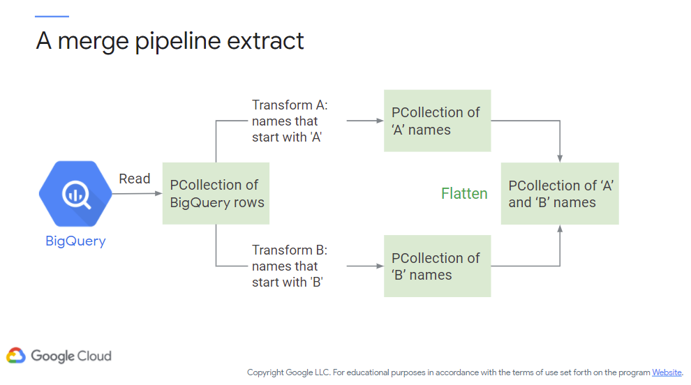
Figure 12: Dataflow - Merge Paths
Are we limited to a single source or sink? Nope! You can feed your pipeline from multiple sources and deposit those PCollections wherever you’d like. You can use internal (to Google Cloud) or external (data feeds) sources to seed your pipeline and transform them as you’d like.
Now let’s take a look at a full example. Figure 13 (c/o Google) shows a full pipeline, reading data from BigQuery and sending it towards Cloud Storage. Transforms along the path include map and reduce operations (to effectively filter and join) – these are fairly common transforms in such an environment. Of interest to you, the cloud developer, is that each step is elastically-scaled. You do not need to create and manage a cluster! Resources are provisioned on demand, rebalanced as necessary, and spun down when done.
Last but not least (for Dataproc/Dataflow at least)…
How do you choose, Dataproc or Dataflow? Figure 14 (c/o Google) shows a decision tree you can use to select the appropriate service:
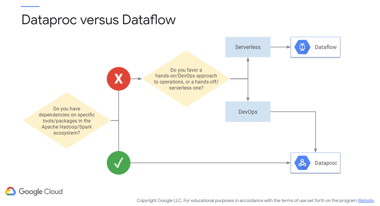
Figure 14: Dataproc vs. Dataflow
Each service can perform the traditional map-reduce operations necessary for big data management. The key difference here is that Dataflow is serverless, whereas Dataproc is more akin to managing a Hadoop/Spark cluster (albeit, as a service).
This video is quite fun…here is the description from the video:
Oh, this was a fun one. I left the majority of me looking foolish in to demonstrate my approach to debugging (I did cut out all the swearing).
Codelab in question: https://codelabs.developers.google.com/codelabs/intro-cloud-composer Notes:
- I had to spin up Composer in the Cloud Shell using gcloud commands (see the Composer manual for details on that), however when actually recording this the GUI worked, so YMMV there.
- There is a problem with the Codelab as is – you need to use n2 machines instead of n1. In Step 4 you can replace n1-standard-1 with n2-standard-2. You also need to edit the Python script that you copy/paste later in that step with the same update (n2-standard-2).
- Module video: Composer/Airflow/Hadoop Demo [30:28]
Lab Choices
Another self-choice! Select one of the following Qwiklabs to get some experience with Dataflow:
BigQuery
First off, watch this video: Google BigQuery - Analytics Data Warehouse (1:58)
Now, let’s take a look at BigQuery. Figure 15 (c/o Google) shows how BigQuery can be used for data warehousing. If you’re not familiar with that term, effectively it is an approach for making business decisions on datasets (and grad-level database classes thrive on such topics).
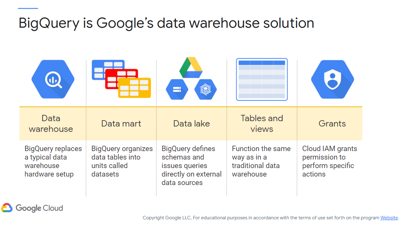
Figure 15: BigQuery Overview
However, if we recall from earlier BigQuery is serverless, meaning you don’t have to deal with that pesky infrastructure. What you see in the above figure are what comprises BigQuery:
- Datasets are just collections of tables divided amongst your analytical domains/business lines/etc. A dataset is tied to a Google Cloud project.
- Data lakes can comprise multiple objects, including Cloud Storage/Google Drive files and Cloud BigTable transactions.
- You can also define a schema for BigQuery to support external data queries
- Tables and views function similarly to a traditional data warehouse – meaning that your (ANSI-2011 compliant) SQL queries are supported
- Cloud IAM can be used to grant/revoke access to BigQuery as with all other services (replacing your traditional SQL
GRANT/REVOKEstatements)
Why BigQuery (or similar) over Data Warehousing
Figure 16 (c/o Google) shows the differences between BigQuery and traditional data warehousing. The biggest takeaway here is that it is serverless and therefore fully managed by Google behind the scenes, so you don’t necessarily need to worry about keeping it up to date.
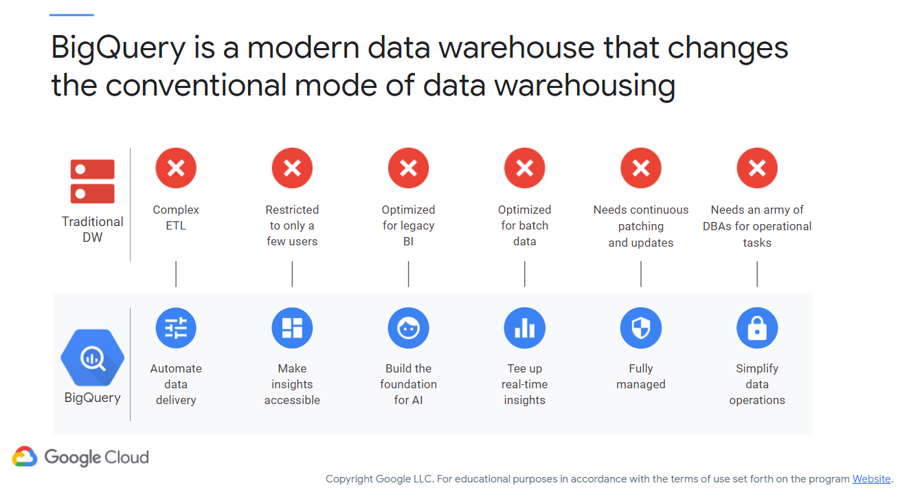
Figure 16: BigQuery vs. Traditional Data Warehousing
One of the nice benefits, aside from traditional warehousing concerns such as business analytics (outside of the scope of this class), is that you can also apply machine learning and artificial intelligence algorithms to datasets within BigQuery – meaning you can perform training and testing on datasets of a massive scale.
As with all other services, resources are available on-demand and are scalable as needed. Again, you pay for what you need.
Loading Data
How do we get data into BigQuery? As we’ve mentioned before, it can come from Cloud Storage, Google Drive files, external sources (assuming they’re federated entities), or even publicly available datasets from Google. You may end up using the gsutil program (a Python application) from the Cloud SDK. This tool lets you talk to Cloud Storage via a command line interface and is quite helpful for BigQuery work. Figure 17 (c/o Google) demonstrates the workflow:
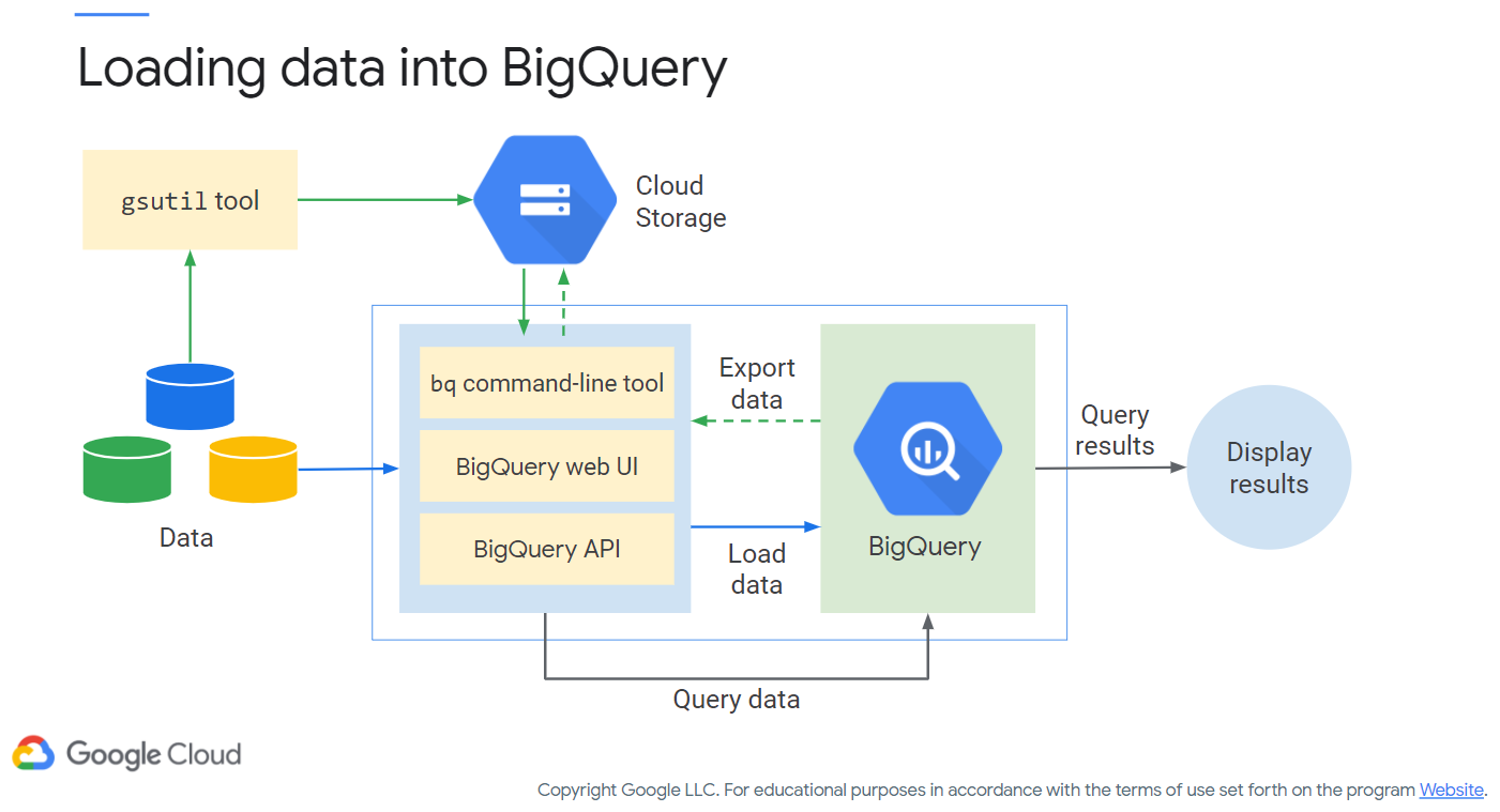
Figure 17: BigQuery Workflow
We’ll play with BigQuery momentarily. However it is worth noting you can use multiple tools for working with BigQuery, external to Google. Figure 18 (c/o Google, oddly enough) shows the tools (currently partnered with Google) you can use.
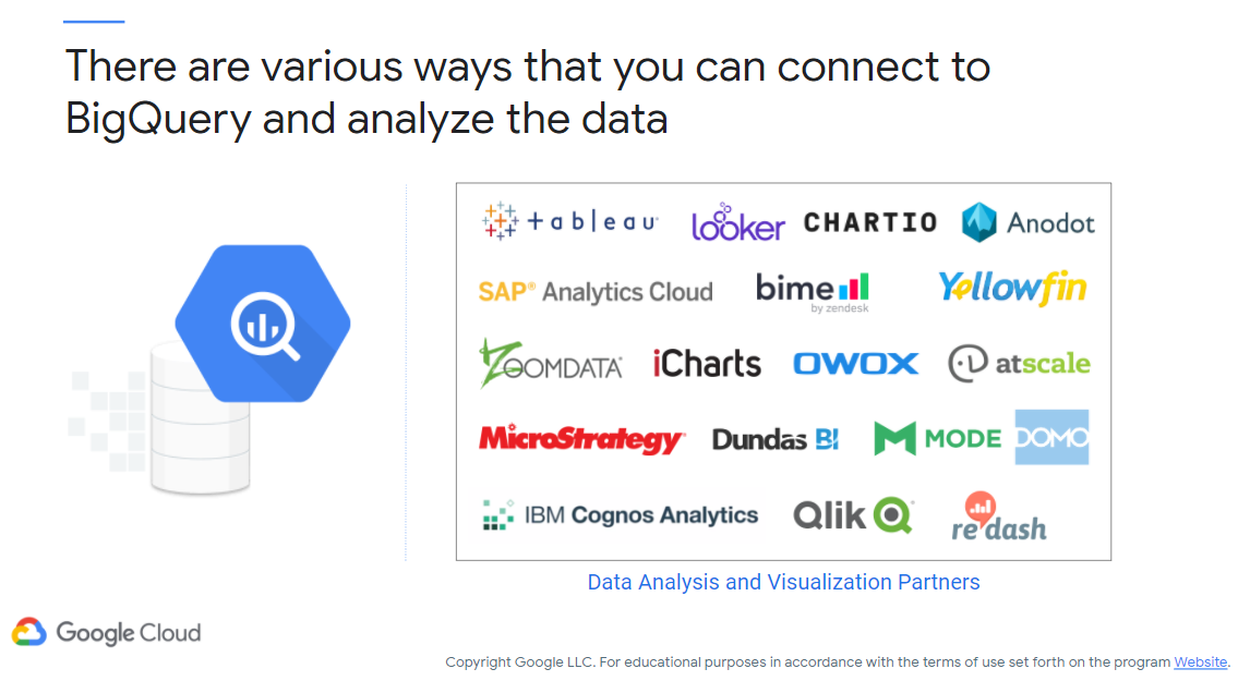
Figure 18: BigQuery Partners
Time for practical experience! No choice here, just do this one!
Additional Resources
- Dataproc
- Amazon analogue = AWS EMR
- Microsoft analogue = Azure Hindsight
- Dataflow
- Amazon analogue = AWS Glue (formerly Data Pipeline)
- Microsoft analogue = Azure Data Factory
- BigQuery
- Amazon analogue = AWS Redshift
- Microsoft analogue = Azure Synapse Analytics
- Hadoop
- Spark
- Dataproc Workflow Templates
- Life of a Dataproc job
- Spark Shell
- Spark Standalone Mode
- Spark Machine Learning Libraries (MLlib)
Where noted, the original content was provided by Google LLC and modified for the purpose of the course, without input or endorsement from Google LLC.